The bard ponders #NoEstimates with some real data
Chris Verhoef and I decided to look for some real project data to explore the value of software estimates and #NoEstimates. We have submitted our research as an article to IEEE for peer review. The complete paper can be found here, and some highly related materials on our prior and ongoing estimation research (M.U.S.E.) can be found here. The following is a summary of the paper.
Abstract: A common approach in agile projects is to use story points, velocity and burnup charts to provide a means for predicting release date or project scope. Another approach that is proposed is to abandon story point estimation and just count stories using a similar burnup chart. We analyzed project data from 55 projects claiming to use agile methods to investigate the predictive value of story point estimation and velocity for project forecasts. The data came from nine organizations ranging from startups to large multinational enterprises. We found that projections based on throughput (story counts) were essentially identical to that of using velocity (story points). Neither velocity nor throughput were great predictors as the uncertainty bands were rather large. Through the use of a simulation model we replicated our findings which aid in understanding the boundary conditions for when story point estimates may be better predictors.
Key Findings
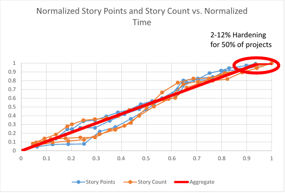
The first thing we noticed was that the normalized burnup charts for Story Points (Velocity) and Story Count (Throughput) were nearly identical. One interesting thing we also found was that roughly 50% of the projects plateaued and required from 2-12% of the total time to finally conclude. We associate that with a probable hardening and/or release readiness period. It is useful to recognize this so that teams can plan accordingly.
So the next thing we looked at was the projection of release date based on the remaining story points using average velocity, or story count using average throughput. To compare the approaches we looked at the P90/P10 ratio as an indicator of range. This ratio is commonly used in domains where the range of the distribution is rather large. The P90 is the 90th percentile and P10 is the 10th percentile. Some domains where it is used frequently are wealth distributions and oil and gas exploration. As a concrete example, the P90/P10 ratio for income inequality is, roughly speaking, the ratio of what professionals like doctors and lawyers earn to what cleaners and fast food workers earn. One of the nice attributes of the P90/P10 ratio is that it uniquely describes the distribution shape for either a lognormal or Weibull distribution.
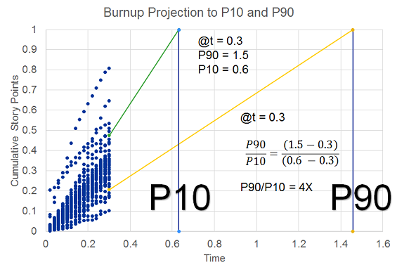
At each iteration we made projections based on the remaining work using the average velocity and throughput. This is a standard approach in agile projects and is mathematically identical to extrapolation using traditional project management Earned Value Management (EVM). We compare these projections against the known actuals to determine the relative errors. The figure below shows the burnup chart for all projects plotted on the same axis scale. In this particular case we have data through t=0.3. Then using the velocity thus far we project out the anticipated release date. The error in the projection is the delta from 1.0. On this same figure we show the P90 and the P10 projections. To determine the actual error bands we subtract out the current projection time (t=0.3). For this chart (with approximations to simplify the math) we have P90 of 1.5, and P10 of 0.6. The revised P90 and P10 are 1.2 and 0.3 respectively, which gives a P90/P10 ratio of 4.0.
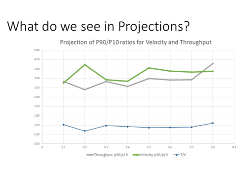
What we discovered was that there was almost no difference in the accuracy band of the velocity projections relative to the throughput projections. In fact the throughput projections were marginally better than the velocity projections. In both cases we found that the accuracy of the projections did not improve as a function of time, consistent with our prior findings about the Cone of Uncertainty [Little] [Eveleens and Verhoef]. Neither velocity nor throughput are particularly good predictors, however, with a P90/P10 ratio on the order of 3.5. In practical terms, whether using velocity or throughput, if a team forecasts that they have about 6 months remaining, the P10 to P90 bands for 80% confidence are roughly 3.2 to 11.2 months. This does not bode well for teams or stakeholders that are expecting estimates that are commitments or even within 25% accurate.
In addition to looking at the raw data, we built a Monte Carlo simulation to explore the impact of Story Point Distribution, Estimation Accuracy, Hardening time, and Estimation Bucketing Approach. We started with the empirical curves from the data and also tried lognormal and Weibull curve fits. The data showed a correlation between Story Points and velocity which we also incorporated in the simulation. We were able to achieve a very good match to the data with overall P90/P10 ratios near 3.5. Once we had this base we were able to run some sensitivity analysis to see what situations resulted in velocity providing improved projections. The simulations showed throughput projections to be essentially identical to velocity projections. One might think that improved estimation accuracy would favor velocity. While velocity projections are improved, the throughput projections are equally improved. The only time we found an advantage to using velocity was when the range of story point distribution is very large. This is good news as the team has a lot to say about how they split their stories so as to reduce the range of the story distribution.
Based on these findings, we made some observations about the implications on critical decisions that teams and organizations make.
| Decisions to steer towards the release | We observed from both the data and the simulations that story point estimates provide minimal improvement in forecasting compared to using throughput for typically observed estimation accuracy. If story point estimates are very accurate (unlikely) then they may provide value. The simulations showed that estimates may also help when there is a large range of story distribution, although an alternative approach would be to split large stories so that the overall distribution is not large. When estimating a container of mixed nuts, we don’t really care too much whether we have smaller peanuts or larger brazil nuts, but we do want to spot any coconuts! |
| Decisions to help with managing iterations | Many teams use detailed task estimation to help them manage their iterations. We did not have access to task estimations for this study, however the findings with story points should be very enlightening. Task estimation and tracking can often be a very time consuming activity. Teams should look at how much value they are getting from these estimations. |
| Decisions at project sanction | Some level of macro-estimation of costs and benefits is likely necessary for business decisions. If the benefits are so overwhelming that it should be done at any cost, then it could be wasteful to spend time on estimating something that does not impact the decision. In general it is waste to spend more time on cost estimation than on benefits. In fact, a study of a number of projects at a major organization found that value generated was negatively correlated to cost forecast accuracy. Too much emphasis on cost or on reduction of uncertainty can destroy forecasting accuracy of value predictions. |
When estimating a container of mixed nuts, we don’t really care too much whether we have smaller peanuts or larger brazil nuts, but we do want to spot any coconuts!

Practitioner’s Guide
Velocity vs. Throughput
With the typically observed story point estimate accuracy range, our results show there is minimal added value to using velocity over using throughput for estimating purposes. When story size distribution is very large, then velocity has better predictive power than throughput.
Hardening
In about half the projects there was a period at the end of the project of between 2-12% of the overall timeline with zero velocity, most likely for release and hardening activities. Unless teams have reasons to believe that they will not require such activities, we recommend either allocating a corresponding time buffer or adding stories (and story points if used) for such activities.
Estimation Accuracy
This study provides additional confirmation that the range of uncertainty with software estimation accuracy is significant and we can confidently say that this range of uncertainty is much larger than many decision makers realize. An interesting finding was that improvements in estimation accuracy helped throughput projections just as much as velocity projections. So while improving estimation accuracy may be a noble goal it is not a reason to favor velocity over throughput.
Bucketing of Estimates
While there was some degradation of the predictive power of velocity as buckets get very large, the overall impact is still very small. Since bucketing approaches are used for expediting estimation processes this finding suggests that teams may continue to use them should they find value in estimating at all. However, we have seen situations where religious adherence to bucketing approaches slowed down or distorted the estimation process and in those circumstances teams may be better suited with simpler approaches. Bucketing or #NoBucketing? You decide.
Uncertainty over Time
Perhaps a bit more bad news for teams and decision makers is that it doesn’t get better over time. The range of relative uncertainty of the work left to be done is large and stays large over time, which is consistent with other findings regarding the Core of Uncertainty.
Decisions
Decisions are being made at multiple levels. For some decisions there may be value to estimates of stories or story points. But those estimates most likely have very large uncertainty ranges. The important question for the team is to understand the decisions they care about, and to comprehend the range of uncertainty to make the appropriate decisions. Decision makers would be wise to learn more about making decisions under uncertainty. There is significant research in many other industries (e.g oil and gas exploration, financial institutions, actuaries, etc.)
Estimates or #NoEstimates
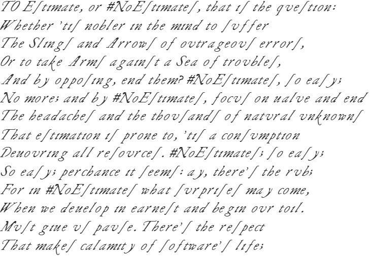
To paraphrase Polonius’ advice to Laertes,


A question on “normalized.” Are the SPs “normalized” between each project. Since SPs are ordinal measures. Is a SP in one project worth the same as a SP in another project?
Hours and dollars are cardinal measures so comparing hours and dollars between projects can be done. How is this done with SPs?
Glen,
Thanks for the question. We aren’t normalizing to compare SP across projects, but rather to compare the overall projects against each other. We normalize SP by dividing by the total SP delivered in the project. We do a similar normalization for time. This ensures that the burnup chart for each project starts at (0,0) and eventually concludes at (1,1). Using this approach allows up to compare projects on the same scale.
Pingback: Dealing with the Quality of Estimates - KBP Media -
Hello Todd,
first of all, thank you for taking the time to create this study!
If I got this right, you conclude that linear extrapolation in the burn up chart doesn’t generate reliable predictions. This confirms my personal experience.
However, the study does not provide evidence that story point estimation is bad in general, nor does it suggest an alternative that creates better results.
Just counting stories doesn’t really reduce estimation effort as you still have to estimate whether a story is a nut or a 10 tons super nut from outer space that has to be split into parts.
Another thing I noticed is that you only used the P90/P10 method without proving in any way that the assumptions for using this method are really met. I’d personally use a few methods just to be sure that the choice of method doesn’t influence the result.
Sebastian,
Thanks for the great post. What I have found is that the use of the linear burnup extrapolation is a good, but not great tool for predictions. For this data using the burnup gives an EQF (Estimation Quality Factor) median of 6.0 for both story point and throughput extrapolation. This compares well with industry data from DeMarco and Lister reporting a median of 3.8. They judged a median EQF of 5.0 as pretty good. I think this improvement in EQF is primarily gained by de-biasing the estimates. That is the one thing that burnups do well, while we frequently see biases with estimates from humans. Burnup charts do not, however, reduce uncertainty unless the underlying data shows such a reduction.
You are correct that this study does not show that story points are bad in general. What we see is that for most conditions, there is little difference between using story points and using throughput. The only condition we studied that showed a significant difference is when the backlog contains stories with a wide distribution of story points. There may be other reasons why story points could be bad or good.
But I would disagree with your contention that counting stories would not reduce estimation time. There is a big difference between quantifying story points for each story and simply identifying which stories are so big that they need to be split.
As for the P90/P10 ratio, I did not post here all the rationale for why we used it. The primary reason that we used it is that it is essentially a means of stating the variance for distributions which are lognormal-ish (lognormal or Weibull). For such skewed distributions, we state the variance as a ratio rather than as a plus/minus which would be proper for a normal symmetric distribution. As we reported, we found the distributions to be close to either lognormal and Weibull. The nice thing about the P90/P10 ratio is that it uniquely describes the shape factor of either a lognormal or a Weibull distribution. For a lognormal distribution, the log of the P90/P10 ratio is proportional to the variance of the log of the distribution. For Weibull it is easy to derive the shape factor from the ratio. In addition to looking at the P90/P10 ratios we also compared the resulting curves visually (they are virtually identical) and also used Q-Q plots.
Lastly, you indicated that you found that burnup chart extrapolations did not produce reliable predictions. I’m curious what approaches you have used that are better.
Todd,
thank you very much for the detailed explanations! The problem I have with linear burnup is that it is a point estimate that doesn’t tell me anything about the uncertainty. It produces a value and I don’t know what to do with it.
We had teams that started slow, the linear burnup indicated a catastrophe and in the end, the projects turned out to be remarkably successful.
We had other teams that started quick and got in trouble close to the end.
Our approach was to try to get the most critical stuff done as early as possible and relied on the people’s judgment (which is far from being perfect of course).
Currently, I’m doing a little research on Monte Carlo estimation (see https://sebastiankuebeck.wordpress.com/2017/03/15/planning-with-uncertainty-part-2/) and I am testing the method by applying it to several open source projects. I’ll publish the results as soon as I’m done.
The nice thing about it is that it doesn’t require assumptions about the distribution and that it produces a distribution instead of a point estimate. The downside is that it requires a reasonable amount of historic data.
To the effort of story point estimation: The of story point estimation depends on the team/company culture. We used Magic Estimation to estimate backlogs with 100+ stories in an hour or so. I have also seen teams who spend a whole day per sprint discussing estimates without getting better results.
Well, if the result is as overwhelming as you wrote than there is no need to verify the method by using a different method. The terrible things that have been done with and to statistics (see e.g. http://journals.plos.org/plosmedicine/article?id=10.1371/journal.pmed.0020124) made me a little bit paranoid. Sorry for that.